This example demonstrates how to log simple plots with the Rerun SDK. Charts can be created from 1-dimensional tensors, or from time-varying scalars.

Used Rerun types

BarChart, Scalar, SeriesPoint, SeriesLine, TextDocument

Logging and visualizing with Rerun

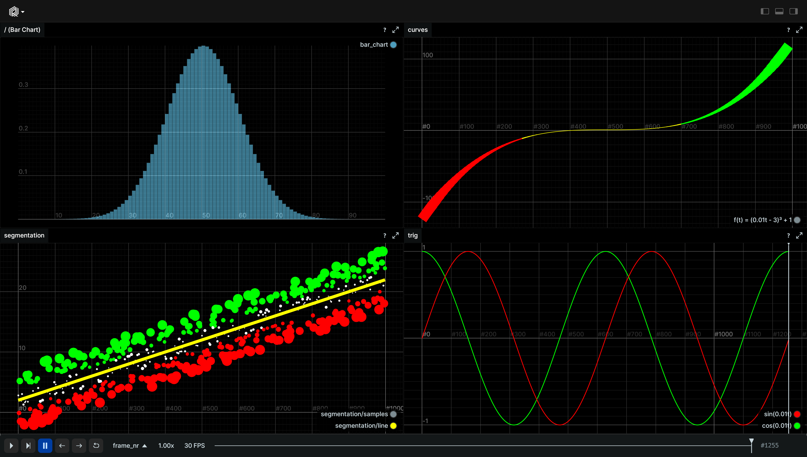
This example shows various plot types that you can create using Rerun. Common usecases for such plots would be logging losses or metrics over time, histograms, or general function plots.

The bar chart is created by logging the BarChart archetype. All other plots are created using the Scalar archetype. Each plot is created by logging scalars at different time steps (i.e., the x-axis). Additionally, the plots are styled using the SeriesLine and SeriesPoint archetypes respectively.

The visualizations in this example were created with the following Rerun code:

Bar chart

The log_bar_chart function logs a bar chat. It generates data for a Gaussian bell curve and logs it using BarChart archetype.

def log_bar_chart() -> None:
    # … existing code …
    rr.log("bar_chart", rr.BarChart(y))

Curves

The log_parabola function logs a parabola curve (sine and cosine functions) as a time series.

It first sets up a time sequence using timelines, then calculates the y-value of the parabola at each time step, and logs it using Scalar archetype. It also adjusts the width and color of the plotted line based on the calculated y value using SeriesLine archetype.

def log_parabola() -> None:
    # Name never changes, log it only once.
    rr.log("curves/parabola", rr.SeriesLine(name="f(t) = (0.01t - 3)³ + 1"), timeless=True)

    # Log a parabola as a time series
    for t in range(0, 1000, 10):
        rr.set_time_sequence("frame_nr", t)

        # … existing code …

        rr.log(
            "curves/parabola",
            rr.Scalar(f_of_t),
            rr.SeriesLine(width=width, color=color),
        )

Trig

The log_trig function logs sin and cos functions as time series. Sin and cos are logged with the same parent entity (i.e.,trig/{cos,sin}) which will put them in the same view by default.

It first logs the styling properties of the sin and cos plots using SeriesLine archetype. Then, it iterates over a range of time steps, calculates the sin and cos values at each time step, and logs them using Scalar archetype.

def log_trig() -> None:
   # Styling doesn't change over time, log it once with timeless=True.
   rr.log("trig/sin", rr.SeriesLine(color=[255, 0, 0], name="sin(0.01t)"), timeless=True)
   rr.log("trig/cos", rr.SeriesLine(color=[0, 255, 0], name="cos(0.01t)"), timeless=True)

   for t in range(0, int(tau * 2 * 100.0)):
       rr.set_time_sequence("frame_nr", t)

       sin_of_t = sin(float(t) / 100.0)
       rr.log("trig/sin", rr.Scalar(sin_of_t))

       cos_of_t = cos(float(t) / 100.0)
       rr.log("trig/cos", rr.Scalar(cos_of_t))

Classification

The log_classification function simulates a classification problem by logging a line function and randomly generated samples around that line.

It first logs the styling properties of the line plot using SeriesLine archetype. Then, it iterates over a range of time steps, calculates the y value of the line function at each time step, and logs it as a scalar using Scalar archetype. Additionally, it generates random samples around the line function and logs them using Scalar and SeriesPoint archetypes.

def log_classification() -> None:
   # Log components that don't change only once:
   rr.log("classification/line", rr.SeriesLine(color=[255, 255, 0], width=3.0), timeless=True)

   for t in range(0, 1000, 2):
       rr.set_time_sequence("frame_nr", t)

       # … existing code …
       rr.log("classification/line", rr.Scalar(f_of_t))

       # … existing code …
       rr.log("classification/samples", rr.Scalar(g_of_t), rr.SeriesPoint(color=color, marker_size=marker_size))

Run the code

To run this example, make sure you have the Rerun repository checked out and the latest SDK installed:

# Setup
pip install --upgrade rerun-sdk  # install the latest Rerun SDK
git clone git@github.com:rerun-io/rerun.git  # Clone the repository
cd rerun
git checkout latest  # Check out the commit matching the latest SDK release

Install the necessary libraries specified in the requirements file:

pip install -r examples/python/plots/requirements.txt

To experiment with the provided example, simply execute the main Python script:

python examples/python/plots/main.py # run the example

If you wish to customize it, explore additional features, or save it use the CLI with the --help option for guidance:

python examples/python/plots/main.py --help