Examples
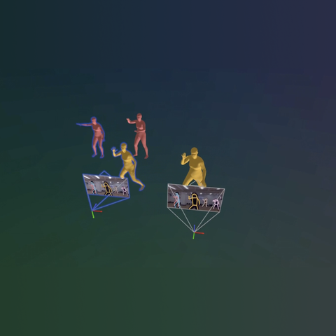
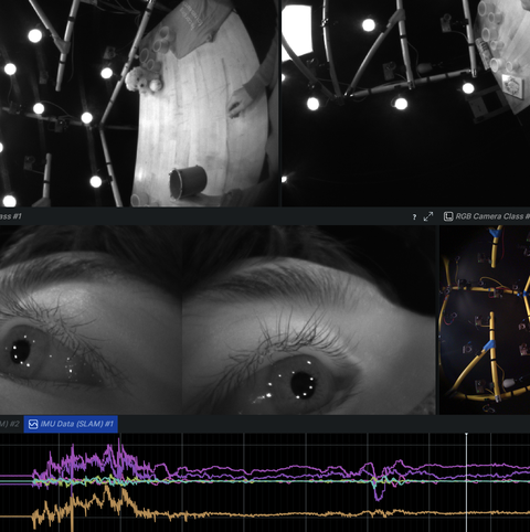
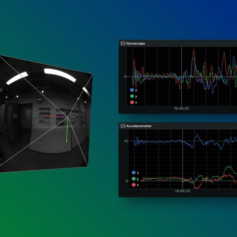
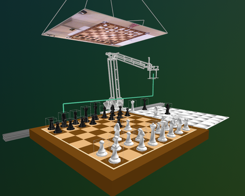
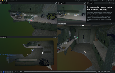
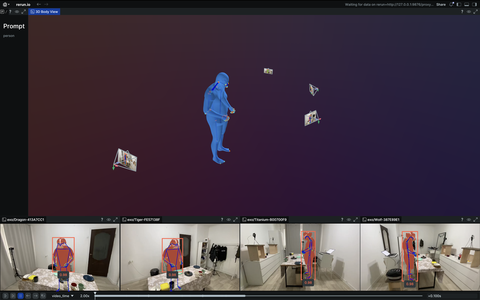
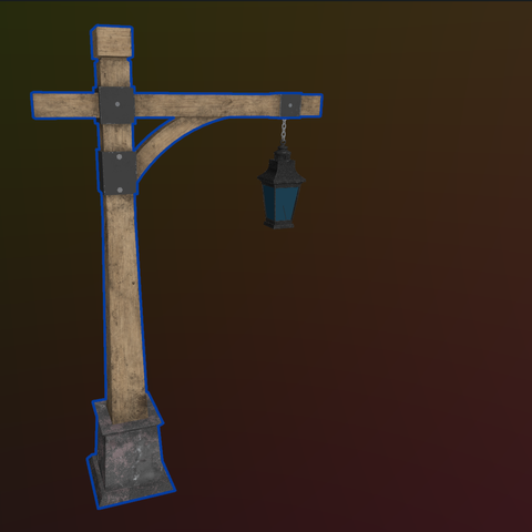
Spatial computing and XR
Examples related to spatial computing, augmented reality, virtual reality, and mixed reality.
- View Source code
- Source code
- Source code
- Source code
- Source code
- Source code
- Source code
- Source code
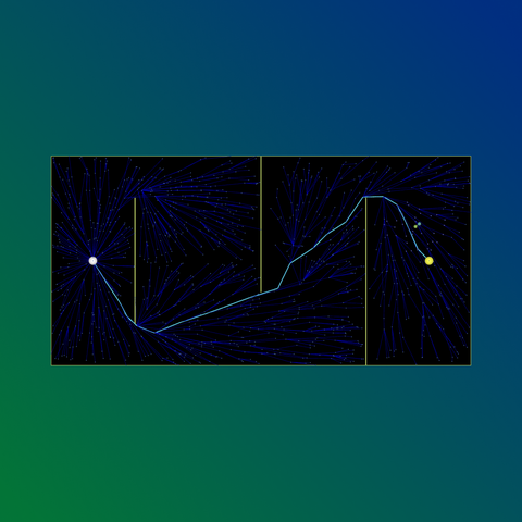
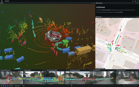
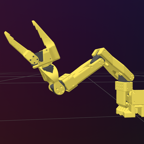
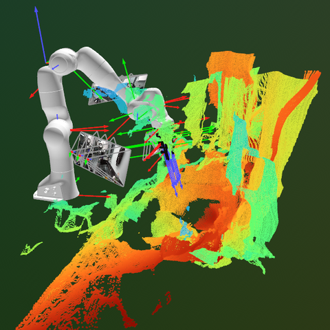
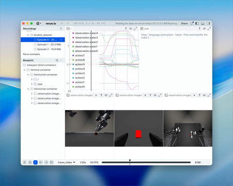
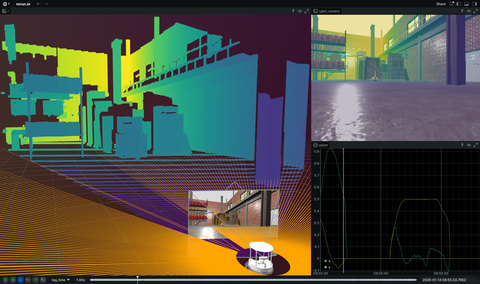
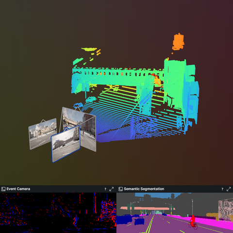
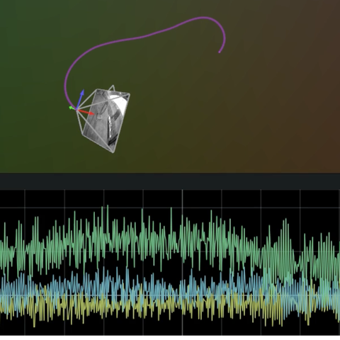
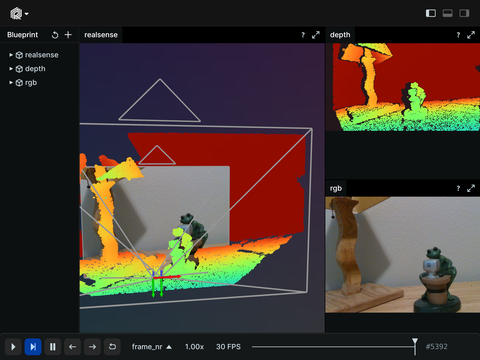
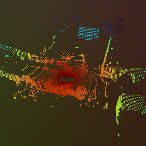
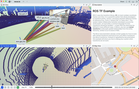
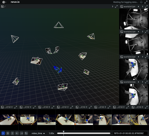
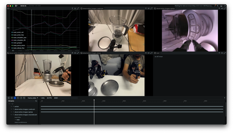
Robotics
Examples related to robotics, autonomous systems, and interfacing with sensor hardware.
- View Source code
- View Source code
- View Source code
- View Source code
- View Source code
- View Source code
- Source code
- Source code
- Source code
- Source code
- Source code
- Source code
- Source code
- Source code
- Source code
- Source code
- Source code
- Source code
- Source code
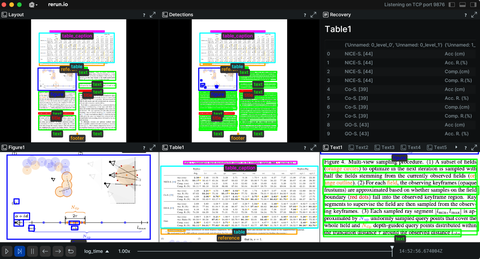
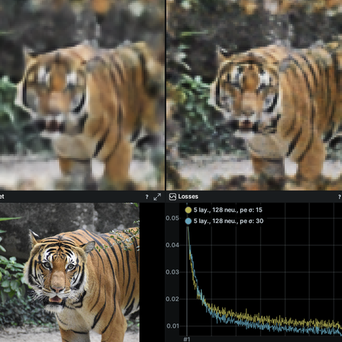
Diffusion models, LLMs, and machine learning
Examples using machine learning and generative AI methods such as diffusion and LLMs.
- Source code
- Source code
- Source code
- Source code
- Source code
- Source code
- Source code
- Source code
- Source code
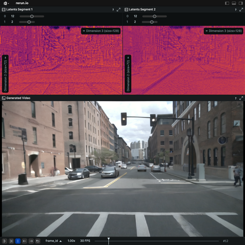
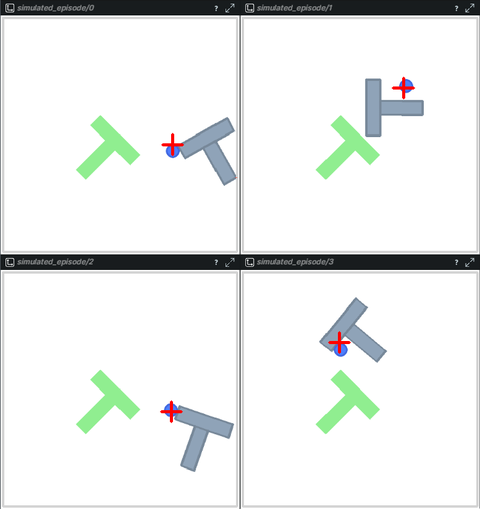
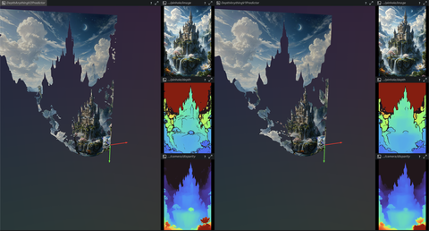
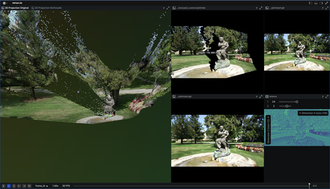
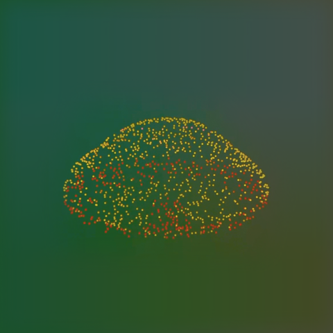
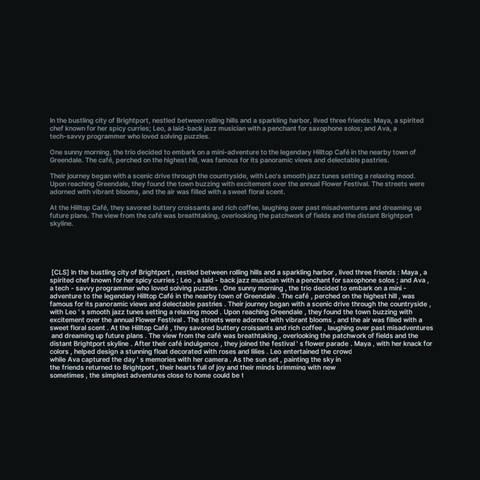
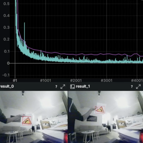
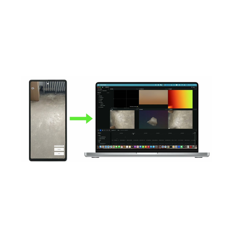
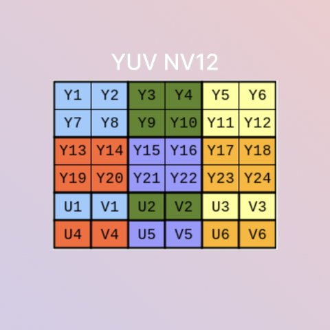
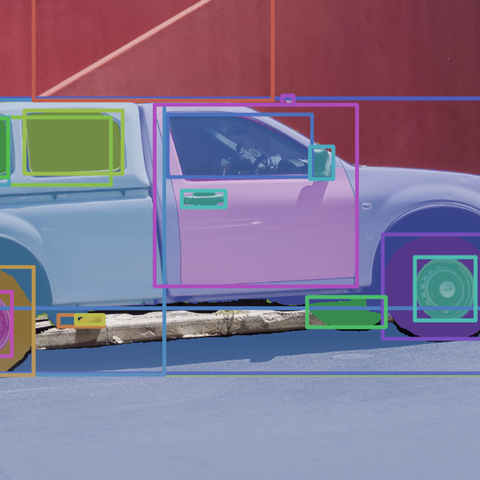
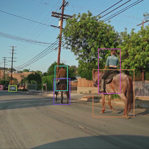
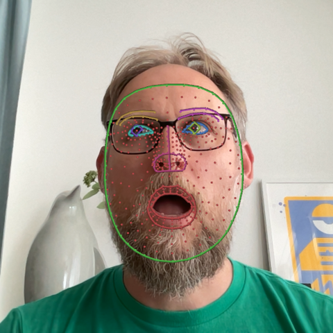
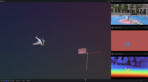
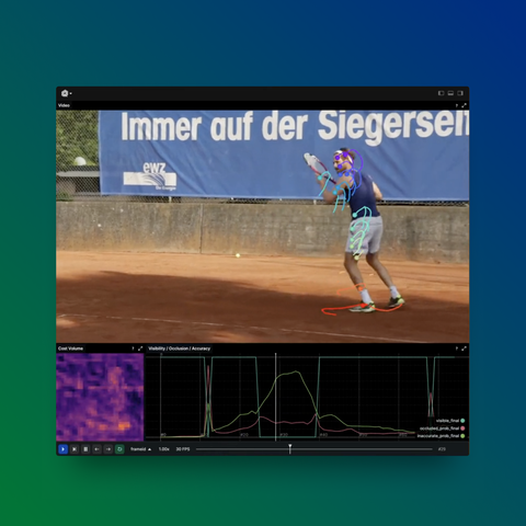
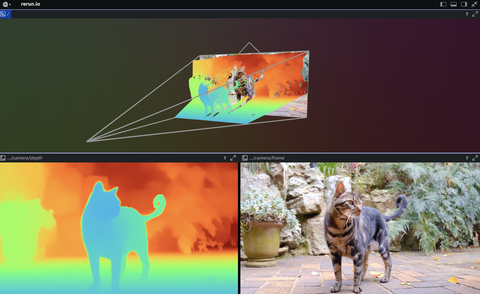
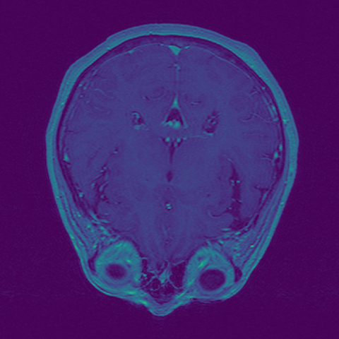
Image and video understanding
Examples related to image and video processing, highlighting Rerun's 2D capabilities.
- View Source code
- View Source code
- Source code
- Source code
- Source code
- Source code
- Source code
- Source code
- Source code
- Source code
- Source code
- Source code
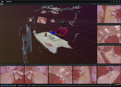
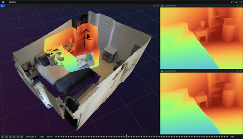

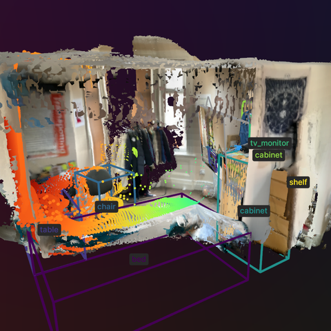
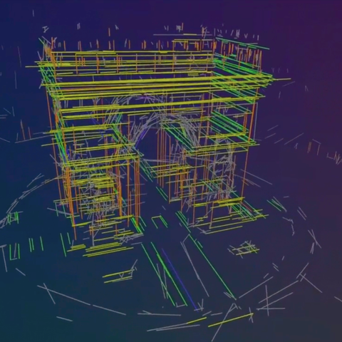
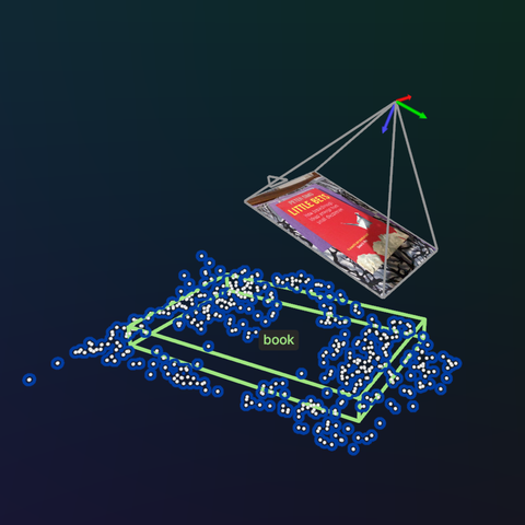
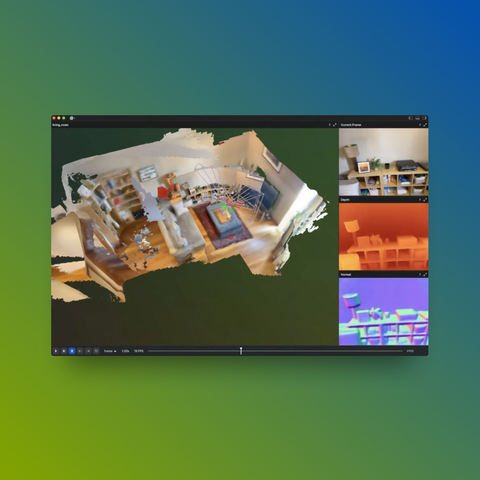
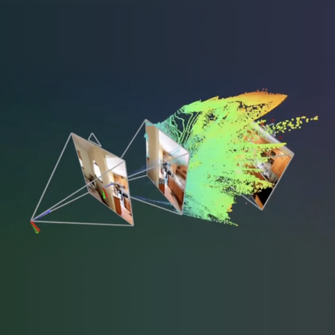
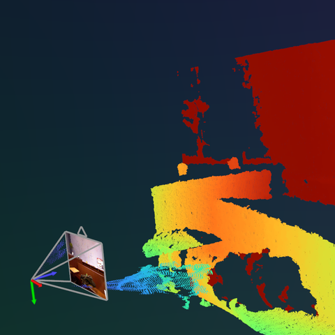
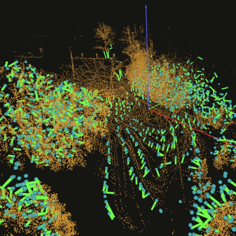
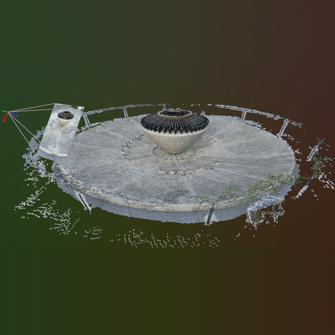
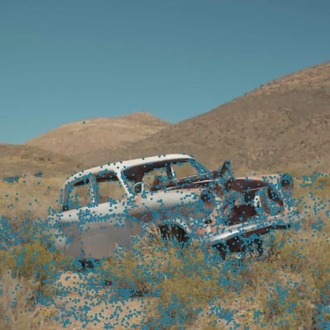
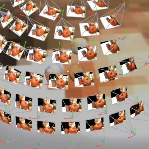
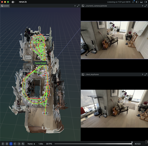
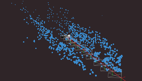
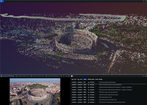
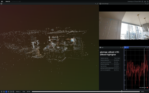
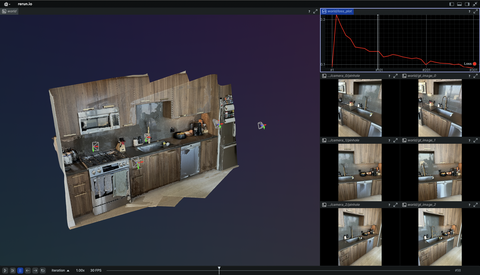
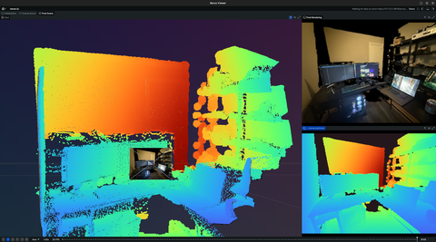
3D reconstruction and modelling
SLAM, photogrammetry and other 3D modelling examples.
- View Source code
- View Source code
- View Source code
- Source code
- Source code
- Source code
- Source code
- Source code
- Source code
- Source code
- Source code
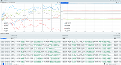
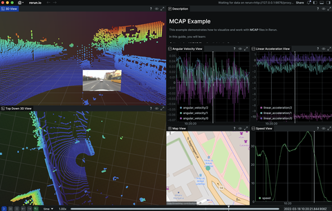
Integrations
Integration with 3rd party tools, formats, libraries, and APIs.
- View Source code
- Source code
- Source code
- Source code
- Source code
- Source code
- Source code
- Source code
- Source code
- Source code
- Source code
- Source code
- Source code
- Source code
- Source code
- Source code
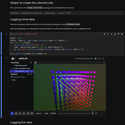
Feature showcase
Showcase basic usage and specific features of Rerun.