In this section we'll log and visualize our first non-trivial dataset, putting many of Rerun's core concepts and features to use.
In a few lines of code, we'll go from a blank sheet to something you don't see every day: an animated, interactive, DNA-shaped abacus:
This guide aims to go wide instead of deep. There are links to other doc pages where you can learn more about specific topics.
The complete code listings for this tutorial live alongside the Rerun source tree: Python, Rust, C++.
Prerequisites
Before starting, make sure you've installed the SDK and set up a project for your language of choice.
Initializing the SDK
Create a new file (or project), import the relevant utilities from your language's SDK, and initialize a recording. Initialization names the recording with a stable ApplicationId, then spawns a Rerun Viewer and connects the recording to it:
from math import tau

import numpy as np

import rerun as rr
from rerun.utilities import bounce_lerp, build_color_spiral
rr.init("rerun_example_dna_abacus", spawn=True)A stable ApplicationId will make the Viewer retain its UI state across runs for this specific dataset, which makes our lives much easier as we iterate.
By default, spawn will start a Viewer in another process and automatically pipe the data through. There are other ways to send data to a Viewer (covered at the end of this section), but the spawn default works great as we experiment.

Logging our first points
The core structure of our DNA-looking shape can easily be described using two point clouds shaped like spirals:
points1, colors1 = build_color_spiral(NUM_POINTS)
points2, colors2 = build_color_spiral(NUM_POINTS, angular_offset=tau * 0.5)

rr.log(
    "dna/structure/left", rr.Points3D(points1, colors=colors1, radii=0.08)
)
rr.log(
    "dna/structure/right", rr.Points3D(points2, colors=colors2, radii=0.08)
)
Run your program and you should now see this scene in the viewer. If the Viewer was still running, Rerun will simply connect to this existing session and replace the data with this new recording.

This is a good time to make yourself familiar with the viewer: try interacting with the scene and exploring the different menus. Checkout the Viewer Walkthrough and viewer reference for a complete tour of the viewer's capabilities.
Under the hood
This tiny snippet of code actually holds much more than meets the eye…
Archetypes
The easiest way to log geometric primitives is to use the SDK's log method with one of the built-in archetype classes (such as Points3D here). Archetypes take care of building batches of components that are recognized and correctly displayed by the Rerun viewer.
Components
Under the hood, the Rerun SDK logs individual components like positions, colors, and radii. Archetypes are just one high-level, convenient way of building such collections of components. For advanced use cases, it's possible to add custom components to archetypes, or even log entirely custom sets of components, bypassing archetypes altogether.
For more information on how the Rerun data model works, refer to our section on Entities and Components. For supplying your own components, see Use custom data.
Entities & hierarchies
Note the two strings we're passing in: "dna/structure/left" & "dna/structure/right".
These are entity paths, which uniquely identify each entity in our scene. Every entity is made up of a path and one or more components. Entity paths typically form a hierarchy which plays an important role in how data is visualized and transformed (as we shall soon see).
Component batches
One final observation: notice how we're logging a whole batch of points and colors all at once. Component batches are first-class citizens in Rerun and come with all sorts of performance benefits and dedicated features. You're looking at one of these dedicated features right now: notice how we're only logging a single radius for all these points, yet somehow it applies to all of them. We call this clamping.
A lot is happening in these two simple function calls. Good news is: once you've digested all of the above, logging any other entity will simply be more of the same. In fact, let's go ahead and log everything else in the scene now.
Adding the missing pieces
We can represent the scaffolding using a batch of 3D line strips:
rr.log(
    "dna/structure/scaffolding",
    rr.LineStrips3D(
        np.stack((points1, points2), axis=1), colors=[128, 128, 128]
    ),
)
Which only leaves the beads:
offsets = np.random.rand(NUM_POINTS)
beads = [
    bounce_lerp(points1[n], points2[n], offsets[n])
    for n in range(NUM_POINTS)
]
colors = [
    [int(bounce_lerp(80, 230, offsets[n] * 2))] for n in range(NUM_POINTS)
]
rr.log(
    "dna/structure/scaffolding/beads",
    rr.Points3D(beads, radii=0.06, colors=np.repeat(colors, 3, axis=-1)),
)
Once again, although we are getting fancier with our array manipulations, there is nothing new here: it's all about populating archetypes and feeding them to the Rerun API.

Animating the beads
Introducing time
Up until this point, we've completely set aside one of the core concepts of Rerun: Time and Timelines.
Even so, if you look at your Timeline View right now, you'll notice that Rerun has kept track of time on your behalf anyway by memorizing when each log call occurred.
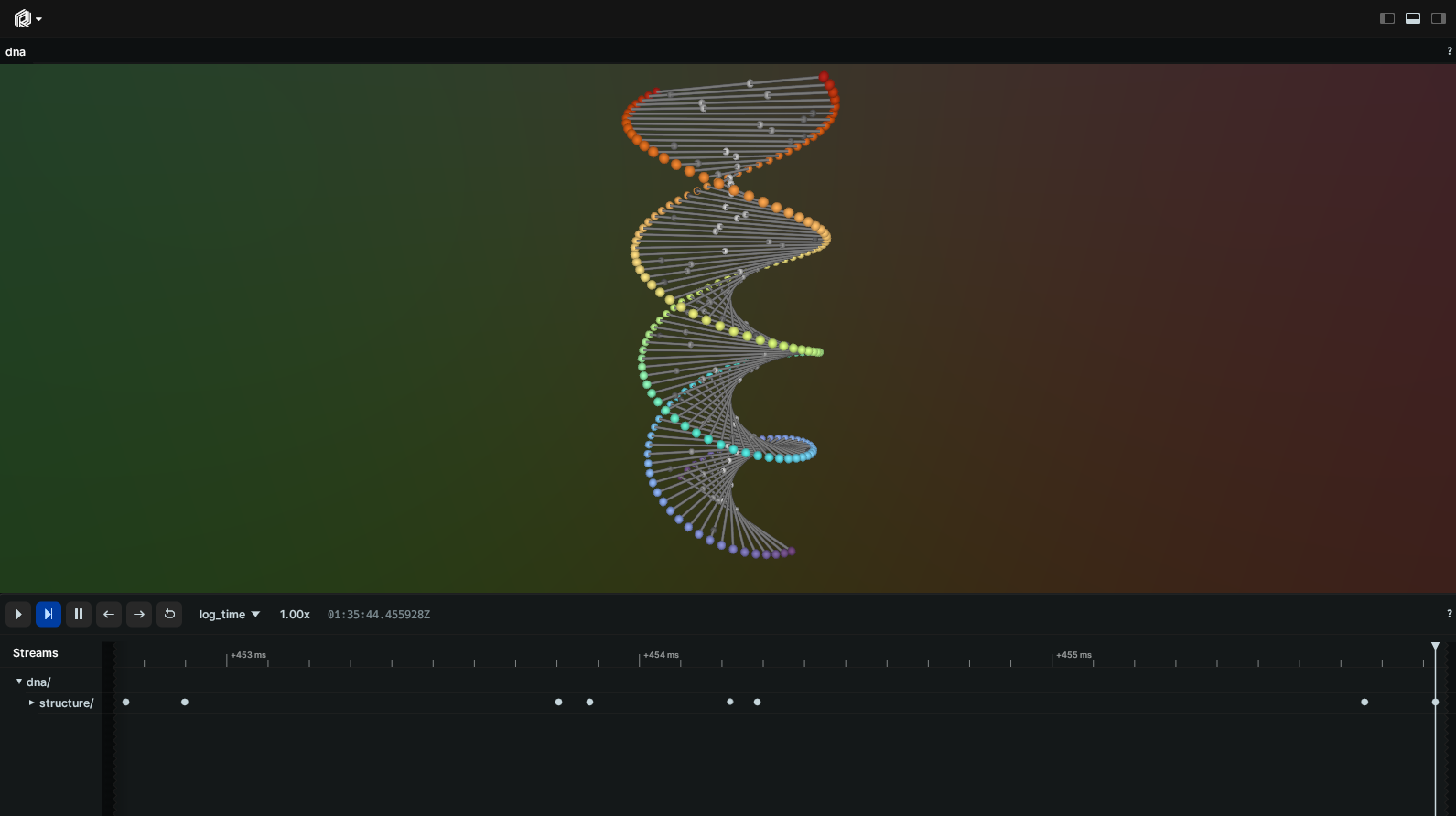
Unfortunately, the logging time isn't particularly helpful to us in this case: we can't have our beads animate depending on the logging time, else they would move at different speeds depending on the performance of the logging process! For that, we need to introduce our own custom timeline that uses a deterministic clock which we control.
Rerun has rich support for time: whether you want concurrent or disjoint timelines, out-of-order insertions or even data that lives outside the timeline(s). You will find a lot of flexibility in there.
Replace the section that logs the beads with a loop that logs them at different timestamps:
for i in range(400):
    time = i * 0.01
    rr.set_time("stable_time", duration=time)

    times = np.repeat(time, NUM_POINTS) + time_offsets
    beads = [
        bounce_lerp(points1[n], points2[n], times[n])
        for n in range(NUM_POINTS)
    ]
    colors = [
        [int(bounce_lerp(80, 230, times[n] * 2))] for n in range(NUM_POINTS)
    ]
    rr.log(
        "dna/structure/scaffolding/beads",
        rr.Points3D(
            beads, radii=0.06, colors=np.repeat(colors, 3, axis=-1)
        ),
    )
A call to set_time (or set_duration_secs in Rust / set_time_duration in C++) creates our new Timeline and makes sure that any logging calls that follow get assigned that time.
You can add as many timelines and timestamps as you want when logging data.
Enter…
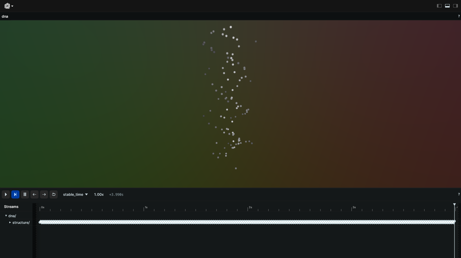
Latest-at semantics
That's because the Rerun Viewer has switched to displaying your custom timeline by default, but the original data was only logged to the default timeline (called log_time).
To fix this, set the custom timeline to time zero before logging the original structure:
rr.set_time("stable_time", duration=0)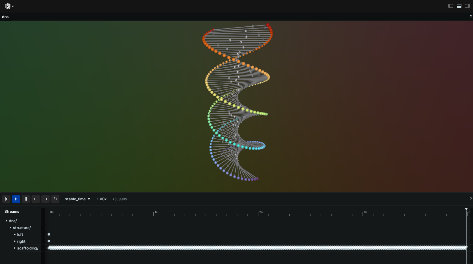
This fix actually introduces yet another very important concept in Rerun: "latest-at" semantics.
Notice how entities "dna/structure/left" & "dna/structure/right" have only ever been logged at time zero, and yet they are still visible when querying times far beyond that point.
Rerun always reasons in terms of "latest" data: for a given entity, it retrieves all of its most recent components at a given time.
Transforming space
There's only one thing left: our original scene had the abacus rotate along its principal axis.
As was the case with time, (hierarchical) space transformations are first-class citizens in Rerun. Now it's just a matter of combining the two: we need to log the transform of the scaffolding at each timestamp.
Either expand the previous loop to include logging transforms or simply add a second loop like this:
for i in range(400):
    time = i * 0.01
    rr.set_time("stable_time", duration=time)
    rr.log(
        "dna/structure",
        rr.Transform3D(
            rotation=rr.RotationAxisAngle(
                axis=[0, 0, 1], radians=time / 4.0 * tau
            )
        ),
    )
Voila!
Other ways of logging & visualizing data
spawn is great when you're experimenting on a single machine like we did in this tutorial, but what if the logging happens on, for example, a headless computer?
Rerun offers several solutions for such use cases.
Logging data over the network
At any time, you can start a Rerun Viewer by running rerun. This Viewer is in fact a server that's ready to accept data over gRPC (it's listening on 0.0.0.0:9876 by default).
On the logger side, replace the spawn call from above with a connect_grpc call to send data to any gRPC address:
"""DNA-abacus example, connecting to a separately-running viewer over gRPC."""

import rerun as rr

rr.init("rerun_example_dna_abacus")
rr.connect_grpc()  # connect to the viewer running at the default URL

# … log data as in the spawn-based example …
Run rerun --help for more options.
Saving & loading to/from RRD files
Sometimes, sending data over the network is not an option. Maybe you'd like to share the data, attach it to a bug report, etc.
Rerun has you covered: each SDK exposes a save method (Python: rr.save, Rust: RecordingStream::save, C++: RecordingStream::save) that streams all logged data to disk. View the resulting file with rerun path/to/recording.rrd.
You can also save a recording (or a portion of it) as you're visualizing it, directly from the viewer.
RRD file backwards compatibility
RRD files saved with Rerun 0.23 or later can be opened with a newer Rerun version. For more details and potential limitations, please refer to our blog post.
Rust-only: showing the Viewer in-process
The Rust SDK can host the Viewer directly inside your application via rerun::native_viewer::show, which expects a complete recording from memory rather than a live stream. This requires enabling the native_viewer feature in Cargo.toml. The Viewer blocks the main thread until closed; see the Rust API docs for details.
Closing
This closes our whirlwind tour of logging with Rerun. We've barely scratched the surface of what's possible, but this should have hopefully given you plenty of pointers to start experimenting.
As a next step, browse through our example gallery for some more realistic example use-cases, browse the Types section for more simple examples of how to use the main datatypes, or dig deeper into querying your logged data.
Opening files
You can also open existing files (RRD, MCAP, images, video, point clouds, etc.) directly with the Viewer — see Opening files.